An introduction to automatic differentiation

Introduction

From allocating wartime resources at the dawn of digital computing in the 1940s, to fitting the parameters of today’s enormous language models, numerical optimization is an ever-present computational challenge. Optimization is nowadays a vast and fascinating subject of applied mathematics and computer science, and there are many excellent introductory texts on it, which I recommend keeping at hand [1,2].

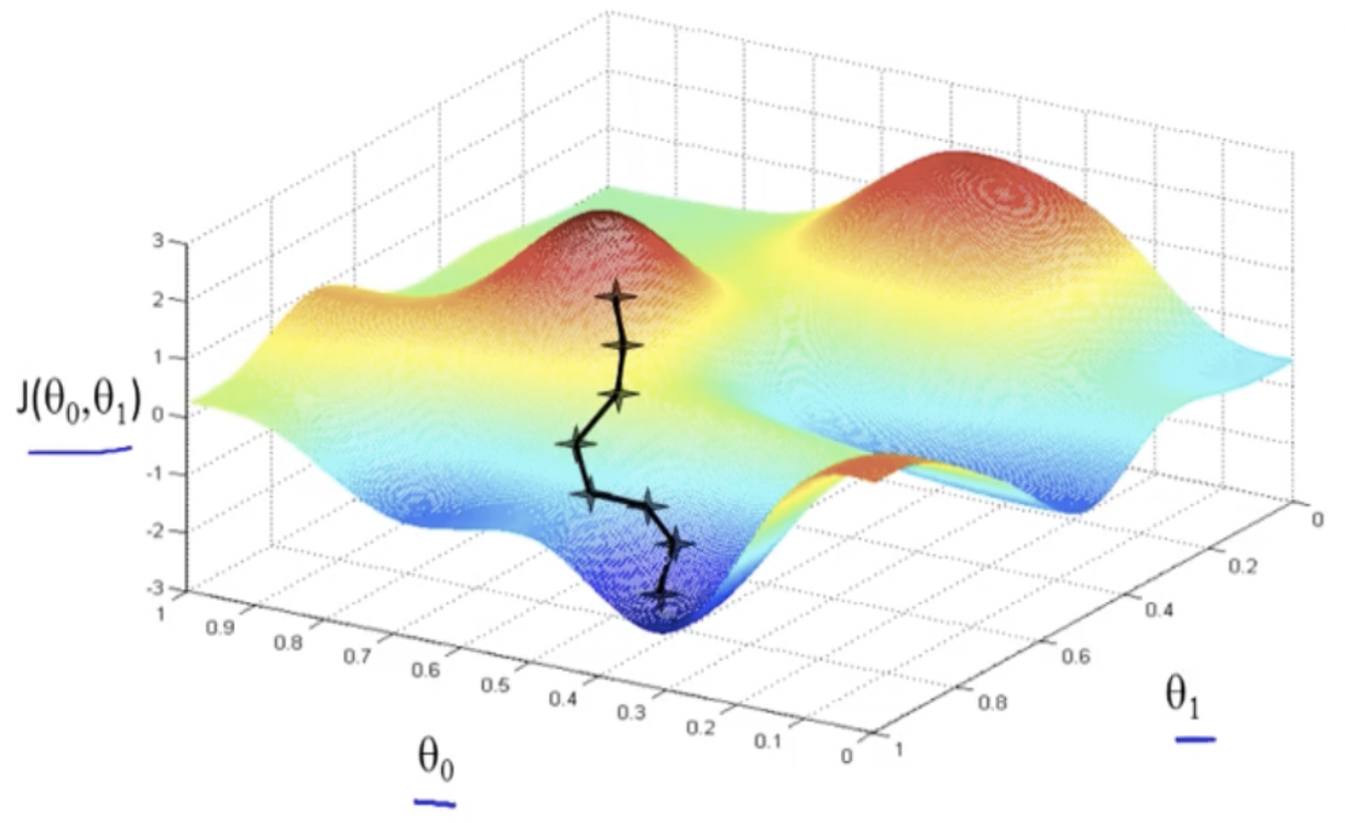
Many real-world optimization problems cannot be solved in closed form, therefore they require iterative improvement of a set of continuous parameters (a parameter vector) with respect to a chosen cost function, and are tackled with some form of gradient descent. The gradient is a vector in parameter space that points to the direction of fastest increase in the function at a given point. The picture above shows a two-parameter cost function \(J(\theta_0, \theta_1)\) evaluated at a fine grid of points and a possible evolution of the gradient descent algorithm.

It’s worth emphasizing that most cost functions of interest are very costly to evaluate, and often have many more parameters than two, making visualization impossible in all but toy examples such as the one above. Computing, and following, the gradient of a cost function implemented as a computer program is then a fundamental and ubiquitous task.

In this post I will give a rather informal account of AD techniques, along with some pointers to literature.

The chain rule

At the highest level of abstraction, a numerical program computes one or more output values from a set of input variables. In the absence of computational “side effects” (e.g. downloading data, querying for user input) and ignoring non-termination, the program can be considered a “pure” function, and its derivatives are readily understood with the tools of elementary calculus.

Suppose we are looking at a composite function \(z(x, y)\), with \(x(u, v)\) and \(y(u, v)\), in which all components are differentiable at least once. The dependencies between these variables can be drawn as a directed acyclic graph :

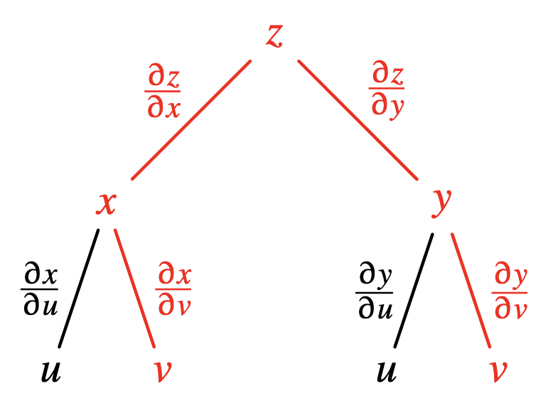
Image from these slides.

The sensitivity of output variable \(z\) to input variable \(v\) must account for all the possible paths taken while “traversing” from \(v\) to \(z\), i.e. while applying the functions at the intermediate tree nodes to their arguments. The multivariate chain rule tells us to sum these contributions : \(\partial_v z = \partial_v x \cdot \partial_x z + \partial_v y \cdot \partial_y z\).

Differentiating computer programs

Automatic differentiation (AD) is a family of techniques that compute the gradient of computer programs, given a program that computes the cost function of interest. This is achieved in two major ways, i.e. while the user program is compiled or as it runs. Source code transformation is an interesting approach that has yielded many successful implementations (from ADIFOR [3] to Jax [4]) but in this post I will focus on the latter formulation.

I emphasize “computer programs” because these contain control structures such as conditionals (if .. then .. else), loops (while), variable mutation and numerous other features which do not appear in mathematical notation and must be accounted for in a dedicated way.

A numerical program is usually built up using the syntactic rules of the host language from a library of elementary functional building blocks (e.g. implementations of the exponential or sine function, exp(), sin(), and so on). This means that computing the overall sensitivity of this program must involve applying the (multivariate) chain rule of differentiation, while accounting for the semantics of the programming language, as outlined above.

When turning theory into practice, one is confronted with multiple implementation details, summarised in this diagram (from [5]) :

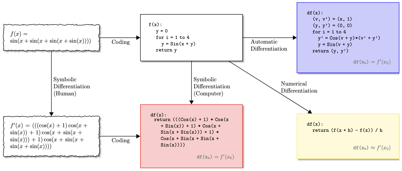
Interested readers who are dissatisfied with my handwaving (there are lots of details under the hood!) might want to refer to [5] for a overview of the design choices that go into an AD system (symbolic vs. numerical vs. algorithmic, compile-time vs. interpreted, forward vs. reverse, etc.).

Forward and Reverse

Ignoring for the sake of brevity all AD approaches that rely on source code transformation, there remain essentially two ways of computing the derivative of a composite function via non-standard evaluation (NSE). By NSE here we mean augmenting the expression variables with adjoint values (thus computing with “dual numbers” [6], i.e. a first-order Taylor approximation of the expression) and potentially modifying the program execution flow in order to accumulate these adjoints (the sensitivities we’re interested in).

Forward-mode AD is the more intuitive of the two approaches : in this case both the expression value(s) at any intermediate expression node \(v_j\) and the adjoints \(\partial_{x_i} v_j\) are computed in the natural reduction order of the expression: by applying function values to their input arguments. Reduction of functions of dual values follows the familiar rules of derivative calculus. The algorithm computes one partial derivative at a time, by setting the dual part of the variable of interest to 1 and all others to 0. Once the expression is fully reduced, \(\partial_{x_i} z\) can be read off the dual part of the result. The computational cost of this algorithm is one full expression evaluation per input variable.

Reverse-mode AD (also called “backpropagation” in the neural networks literature) achieves the same result by tracking the reduction order while reducing the expression (“forward”), initializing all duals to \(0\), and accumulating the adjoints “backwards” from the output variable \(z\), which is initialized with the trivial adjoint \(\partial_z z = 1\). Each expression node represents a function, and it is augmented (“overloaded”, in programming language terminology) with a pullback [7] that computes how input sensitivities change as a function of output sensitivities. Upon returning to a given expression node \(v_i\), its adjoints are summed over (following the multivariate chain rule shown in a previous paragraph). In this case, all parameter sensitivities are computed at once at the end of the backwards sweep. The cost of reverse-mode AD is two full expression evaluations per output variable, which might save a lot of work when applied to expressions with many more input variables, as often happens in optimization and machine learning.

Both AD modes have a long history of successful implementations. Many implementations of reverse-mode AD “reify” the user function into a data structure that tracks the execution history and the functional dependencies (a “Wengert tape”), in order to play the program backwards when accumulating the adjoints.

Program reification is not the only way to implement reverse-mode AD. In an upcoming blog post I will show a purely-functional approach based on delimited continuations which is both elegant and efficient.

Discussion

Automatic differentiation gained widespread adoption in the recent years; it embodies relatively simple ideas but requires some care in implementation. I hope this post has clarified (or at least demystified) the principles behind these tools, and can serve to inspire the next generation of AD frameworks.

References

[1] Nocedal, Wright - Numerical Optimization

[2] Boyd, Vanderberghe - Convex Optimization - https://web.stanford.edu/~boyd/cvxbook/

[3] ADIFOR - https://www.anl.gov/partnerships/adifor-automatic-differentiation-of-fortran-77

[4] Jax - https://github.com/google/jax

[5] Baydin, Pearlmutter - Automatic differentiation of machine learning algorithms - https://arxiv.org/abs/1404.7456

[6] Shan - Differentiating regions - http://conway.rutgers.edu/~ccshan/wiki/blog/posts/Differentiation/

[7] Innes - Don’t unroll adjoint : Differentiating SSA-form programs - https://arxiv.org/abs/1810.07951